Model summaries for a Bayesian linear regression

The packages mmcc creates tidy summaries of Bayesian models, in the fashion of broom, with one important difference - mmcc uses a data.table instead of a tibble, due to the size of the output that is all too easily possible in Bayesian models.

The aim of this vignette is to demonstrate how to use the two key functions of mmcc, mcmc_to_dt() and tidy (which actually calls mmcc:::tidy.mcmc.list under the hood).

First, we simulate some data to fit a Bayesian model to.

set.seed(4000)
N <- 20
x <- sort(runif(n = N))
y <- rnorm(n = N, 
           mean = 2*x + 1, 
           sd = 0.25)
dat <- data.frame(x = x, y = y)

library(ggplot2)
ggplot(data = dat,
       aes(x = x, 
           y = y)) +
    geom_point() +
    theme_bw()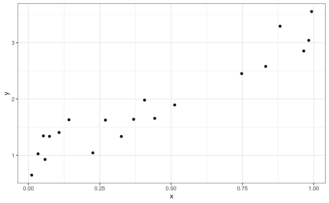

Then, we simulate some values for predicting

M <- 10
x_pred <- seq(from = min(x), 
              to = max(x), 
              length.out = M)

Next, we fit the model, specified as

jags_model <- 
"model{
    # model block
    for (i in 1:n){
        y[i] ~ dnorm(mu[i], tau_y)
        mu[i] <- beta_0 + beta_1*x[i]
    }

    # prediction block
    for (i in 1:m){
        y_pred[i] ~ dnorm(mu_pred[i], tau_y)
        mu_pred[i] <- beta_0 + beta_1*x_pred[i]
    }

    # priors
    beta_0 ~ dunif(-1e12, 1e12)
    beta_1 ~ dunif(-1e12, 1e12)
    tau_y <- exp(2*log_sigma)
    log_sigma ~ dunif(-1e12, 1e12)
}"

and then generate the mcmc_object with the rjags package.

library(rjags)
#> Loading required package: coda
#> Linked to JAGS 4.2.0
#> Loaded modules: basemod,bugs
model <- jags.model(file = textConnection(jags_model),
                    data = list(n = N,
                                x = x,
                                y = y,
                                m = M,
                                x_pred = x_pred),
                    n.chains = 3)
#> Compiling model graph
#>    Resolving undeclared variables
#>    Allocating nodes
#> Graph information:
#>    Observed stochastic nodes: 20
#>    Unobserved stochastic nodes: 13
#>    Total graph size: 131
#> 
#> Initializing model

We draw burn-in samples and posterior inference samples for all terms in the model.

burn <- jags.samples(model = model,
                     variable.names = c("beta_0", 
                                        "beta_1", 
                                        "tau_y", 
                                        "mu"),
                     n.iter = 5000)

samples <- coda.samples(model = model,
                        variable.names = c("beta_0", 
                                           "beta_1", 
                                           "tau_y", 
                                           "mu_pred", 
                                           "y_pred"),
                        n.iter = 10000)

We can now convert the posterior samples to a data.table and summarise the regression parameters. A data.table object is very useful in this case when you have many samples for many parameters.

library(mmcc)

# convert to a data.table
samples_dt <- mcmc_to_dt(samples)
samples_dt
#>         iteration chain  parameter     value
#>      1:         1     1     beta_0 0.9112238
#>      2:         2     1     beta_0 0.8010436
#>      3:         3     1     beta_0 0.8643769
#>      4:         4     1     beta_0 0.7944889
#>      5:         5     1     beta_0 0.8408893
#>     ---                                     
#> 689996:      9996     3 y_pred[10] 3.5722373
#> 689997:      9997     3 y_pred[10] 3.3416762
#> 689998:      9998     3 y_pred[10] 3.0006974
#> 689999:      9999     3 y_pred[10] 3.3961728
#> 690000:     10000     3 y_pred[10] 3.3583402

pars_dt <- tidy(samples, 
                conf_level = 0.95, 
                colnames = c("beta_0", 
                             "beta_1", 
                             "tau_y"))

pars_dt
#>    parameter      mean        sd      2.5%    median     97.5%
#> 1:    beta_0  0.924492 0.0994490 0.7262698  0.923934  1.121158
#> 2:    beta_1  2.225250 0.1834351 1.8637230  2.226307  2.585992
#> 3:     tau_y 13.782520 4.5543831 6.3572410 13.303498 24.008296

Summarise the line of best fit, mu, and the predictions, y_pred,

mu_dt <- tidy(samples, 
              conf_level = 0.95, 
              colnames = "mu_pred")

y_dt <- tidy(samples, 
             conf_level = 0.95, 
             colnames = "y_pred")

For plotting, we add the prediction \(\boldsymbol{x}\) values to these data tables.

mu_dt[ , x:= x_pred]
y_dt[ , x:= x_pred]
y_dt
#>      parameter      mean        sd      2.5%    median    97.5%         x
#>  1:  y_pred[1] 0.9478433 0.3002920 0.3506615 0.9463829 1.543704 0.0112199
#>  2:  y_pred[2] 1.1934373 0.2980774 0.6011571 1.1921787 1.788495 0.1202395
#>  3:  y_pred[3] 1.4349571 0.2944812 0.8523959 1.4342498 2.023439 0.2292590
#>  4:  y_pred[4] 1.6742918 0.2935478 1.0907819 1.6740384 2.257015 0.3382786
#>  5:  y_pred[5] 1.9206716 0.2941172 1.3418086 1.9225791 2.500972 0.4472982
#>  6:  y_pred[6] 2.1638978 0.2947522 1.5818237 2.1642891 2.750502 0.5563177
#>  7:  y_pred[7] 2.4055666 0.2966433 1.8186290 2.4031570 2.997888 0.6653373
#>  8:  y_pred[8] 2.6480627 0.2998802 2.0558604 2.6485508 3.246963 0.7743569
#>  9:  y_pred[9] 2.8927452 0.3072666 2.2852859 2.8905180 3.509767 0.8833765
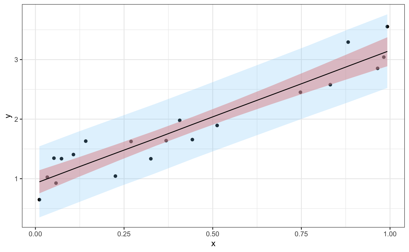
#> 10: y_pred[10] 3.1366084 0.3113266 2.5240160 3.1354399 3.759669 0.9923960

Now we’ll generate a plot that shows the data, a 95% credible interval for the predictions, \({\hat{\bm{y}}}_{pred}\), and a 95% credible interval for their means, \({\hat{\bm{\mu}}}_{pred}\).

If we tidy the samples object, we can look at the distribution of values

tidy_samples <- mcmc_to_dt(samples, 
                           colnames = c("beta_0", 
                                        "beta_1", 
                                        "tau_y"))

ggplot(data = tidy_samples, 
       aes(x = value)) +
    geom_density(color = "black", 
                 fill = "grey90") +
    facet_wrap(~parameter,
               nrow = 1,
               scales = "free") +
    theme_bw() +
    geom_segment(data = pars_dt,
                   aes(x = `2.5%`,
                       xend = `97.5%`),
                 y = 0, 
                 yend = 0,
                 size = 2) +
    geom_point(data = pars_dt,
               aes(x = mean),
               y = 0,
               color = "white")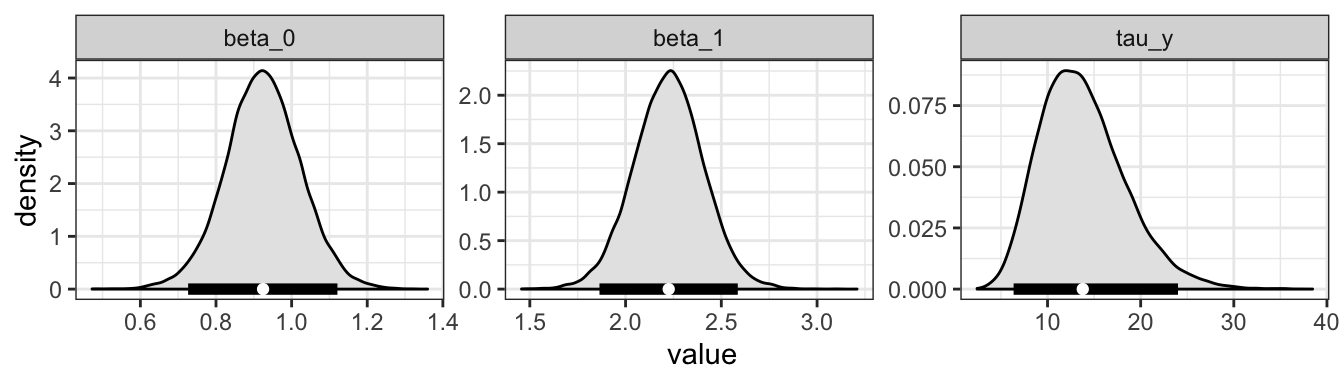

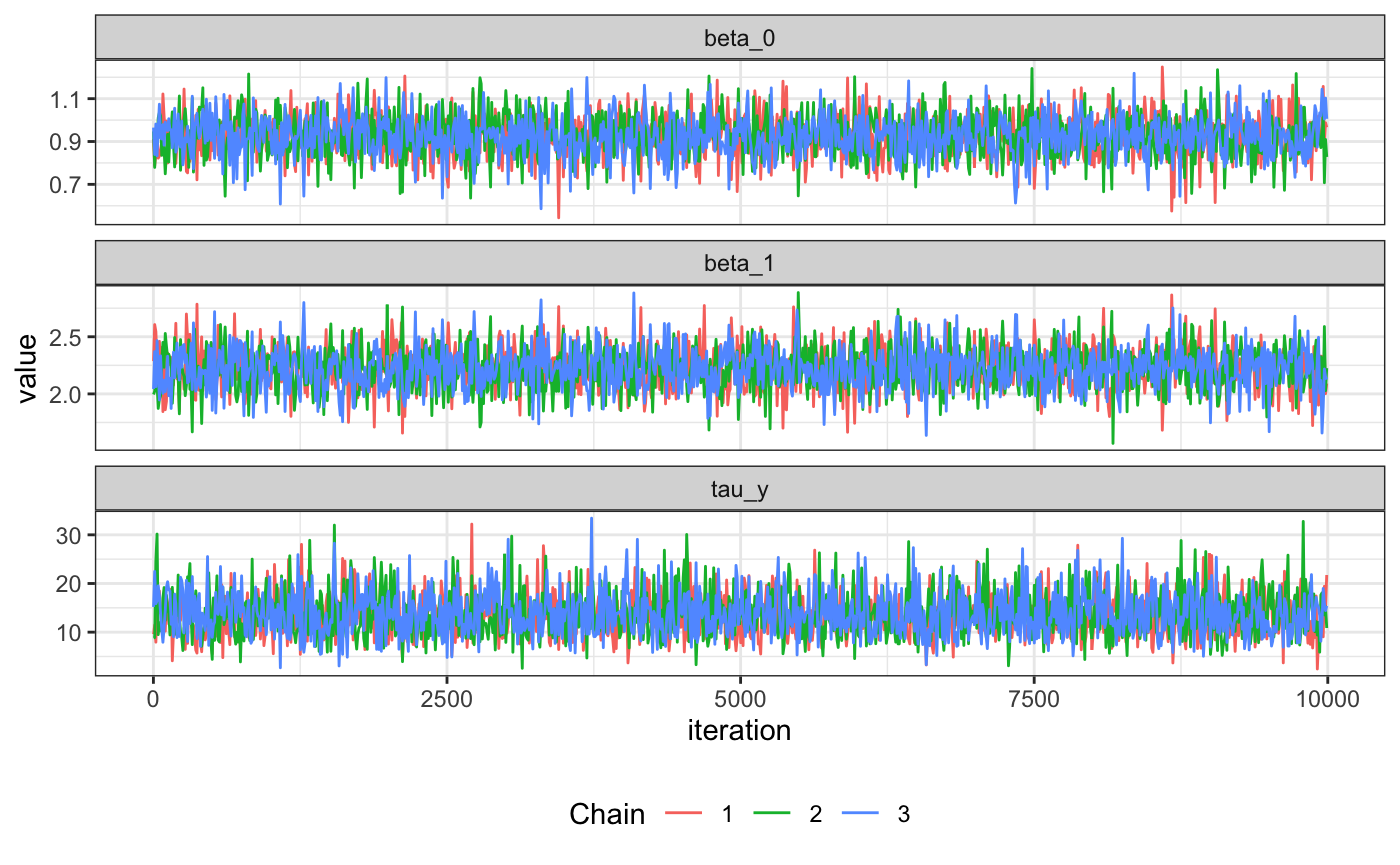
We can also thin to create trace plots and plot per chain

tidy_samples_10 <- thin_dt(tidy_samples, thin = 10)

ggplot(data=tidy_samples_10, aes(x=iteration, y=value)) +
    geom_line(aes(group=chain, color=factor(chain))) +
    facet_wrap( ~ parameter, ncol=1, scales="free_y") +
    theme_bw() +
    theme(legend.position = "bottom") +
    scale_color_discrete(name="Chain")

Sam Clifford

2019-02-01